Custom Pipelines in Kubeflow
How to create a Pipeline Notebook?
1. Navigate to the "Notebooks" page of Kubeflow and press + New Notebook
A page like the following will be displayed:
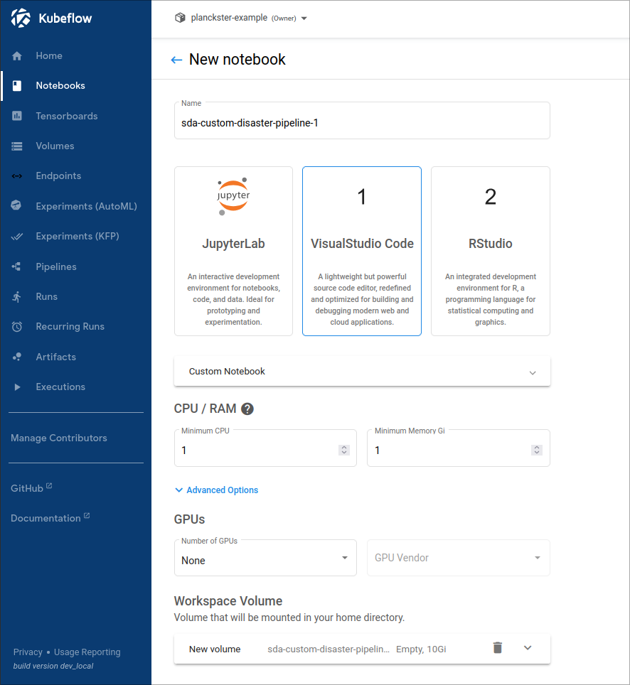
2. When you are in the New Notebook page you will:
- Select a descriptive name for the notebook
- Select VisualStudio Code as the editor for the notebook
- Select an appropriate amount of CPU and RAM for the pipeline
- Add more storage to the volume if needed
- Check Allow access to Kubeflow Pipelines in the Configurations dropdown. This step is critical to allow this notebook to create a new (custom) pipeline.
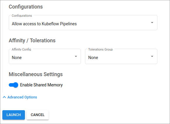
- Click Launch
How to create a new DAG with existing pipeline elements?
1. Create and setup the .ipynb Notebook
!pip install kfp==1.8.22
import kfp
from kfp import compiler, dsl

kfp.Client() # this can be used to test if the connection is successful
Note: We use kfp version 1.8.22 throughout our entire Kubeflow instance, Compatibility >2.0.0 versions will arrive in v3.
Example:
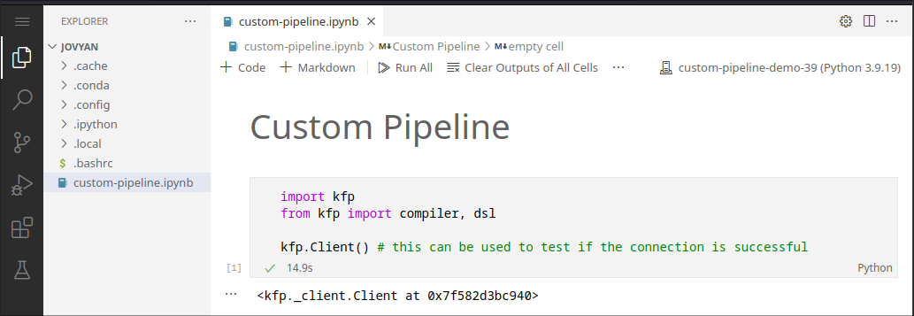
- Create a new .ipynb notebook within the home folder of the default user (Jovyan)
- Select a python kernel, ideally a new conda environment.
- Install the "kfp" python package (allows connecting to Kubeflow client)
2. Loading components
In general, components can be loaded and reused using the following code:
component = kfp.components.load_component_from_file("./component.txt")
Example:
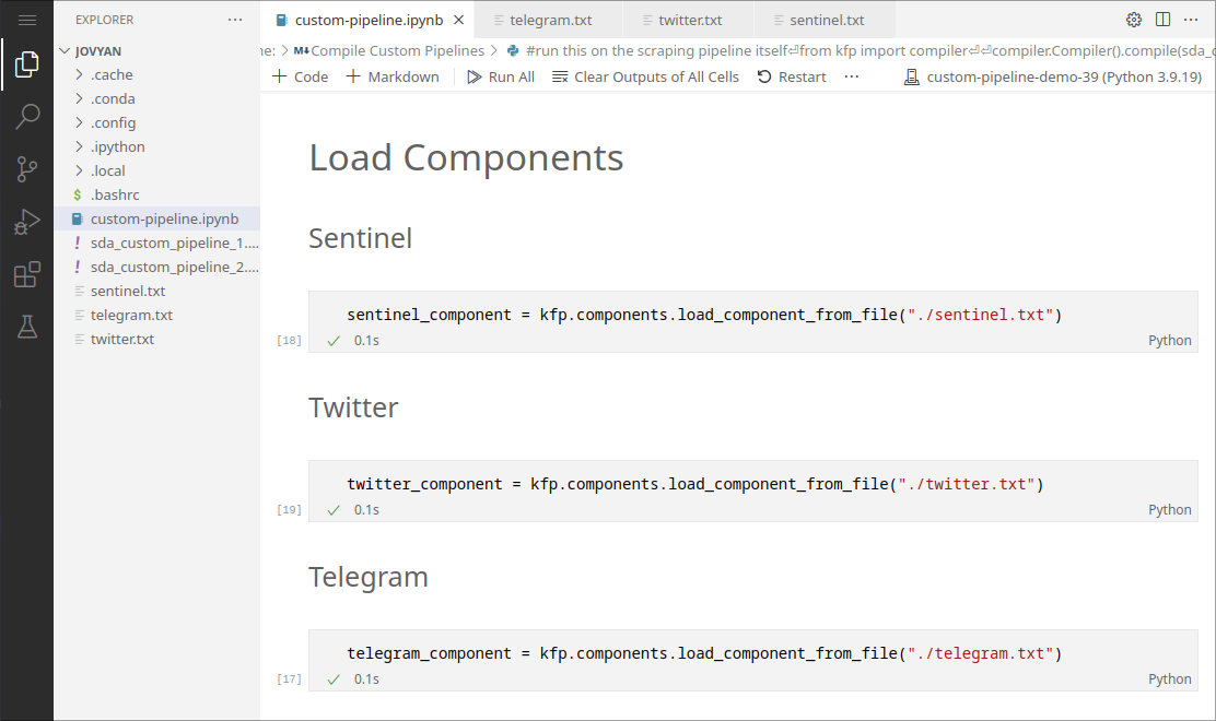
We can load the sentinel, twitter, and telegram components defined in the original SDA-disaster-scrapers.ipynb" notebook. This avoids having to redefine the long wrapper functions for these components.
Note: This functionality requires components to be saved to a .txt file: see the next section
3. Saving Components
In general, components can be saved with the following code after component_wrapper is defined:
# save component
with open("./components/component.txt", "w") as text_file:
    text_file.write(func_to_component_text(component_wrapper, base_image="maany/mpi-sda-component:version"))
Example:
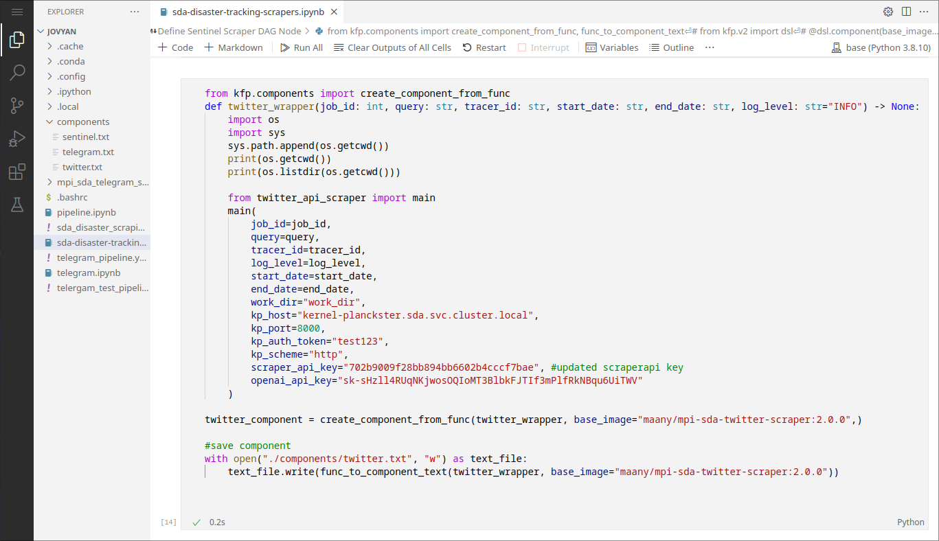
This is how we save components to .txt files in the original sda-disaster-scrapers.ipynb notebook.
4. Assemble Custom Pipelines
In general, custom pipelines are assembled as a set of tasks with execution options:
def custom_pipeline_1(INPUT PARAMETERS): # Input Parameters can be adjusted in the Kubeflow UI

    # parallel execution:
    component1_scraping_task = component1(ARGUMENTS)
    component1.execution_options.caching_strategy.max_cache_staleness = "P0D"

    component2_scraping_task = component2(ARGUMENTS)
    component2.execution_options.caching_strategy.max_cache_staleness = "P0D"
Example:
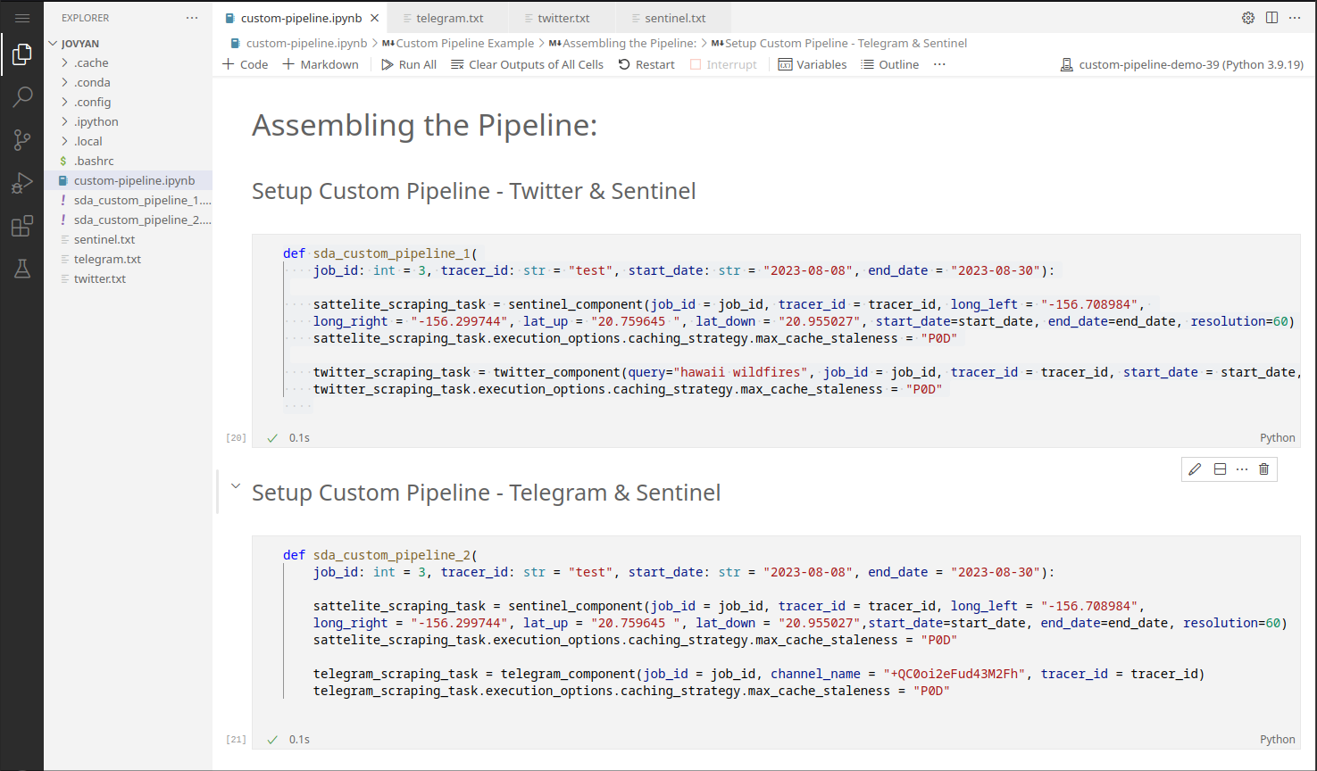
5. Compile Custom Pipelines
In general, custom pipelines are compiled to a .yaml file which is then uploaded to Kubeflow:
from kfp import compiler

#save the pipeline locally
compiler.Compiler().compile(custom_pipeline_1, package_path='custom_pipeline_1.yaml')

#upload and register the pipeline with Kubeflow
kfp.Client().upload_pipeline(
    'custom_pipeline_1.yaml',
    pipeline_name="custom_pipeline_1-VERSION",
)
Example:
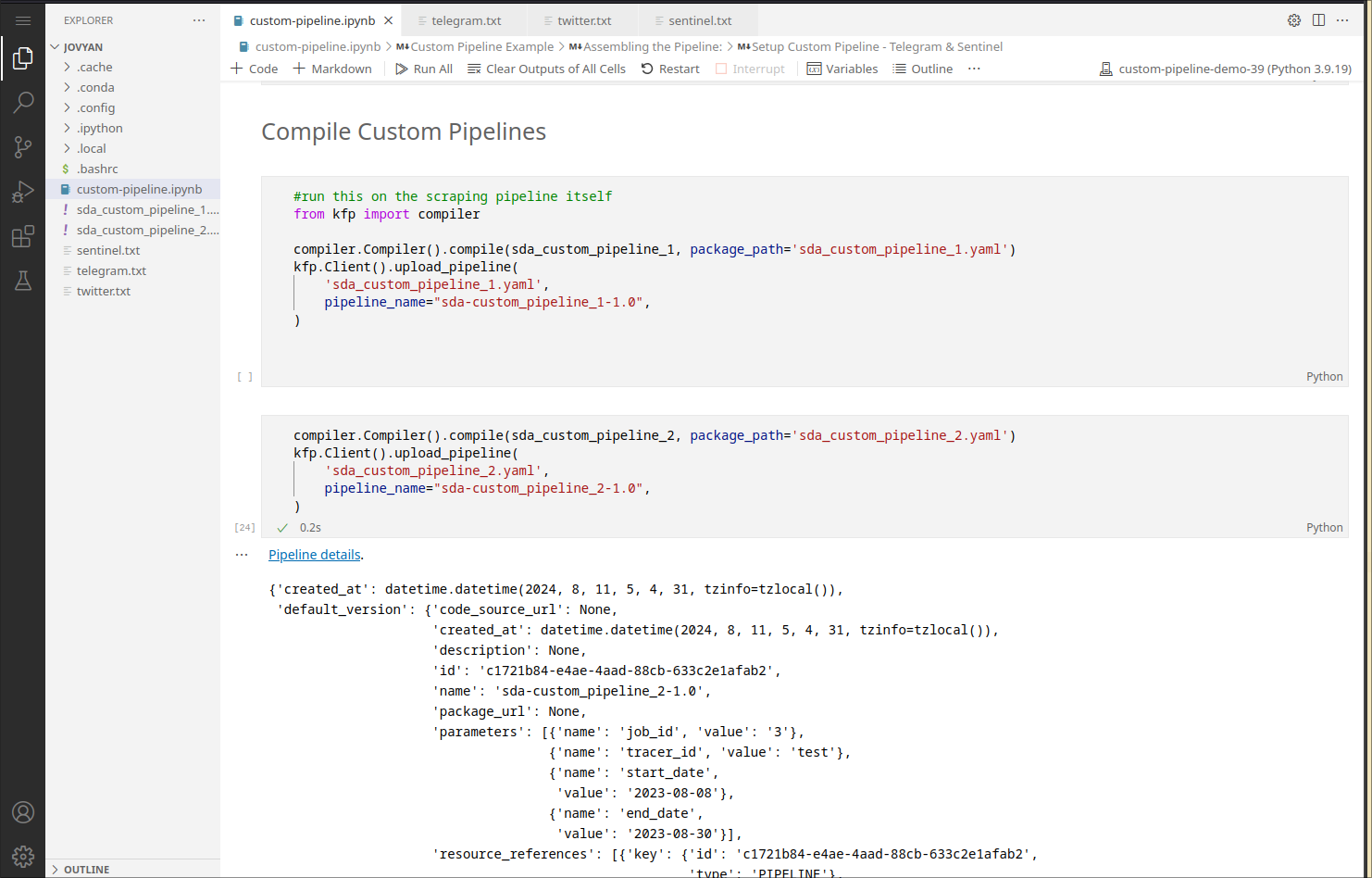
Note that a pipeline can only be uploaded once with the same version. To reupload, bump up the version number in the pipeline_name option when compiling.
How to create a run for the pipeline?
1. Navigate to the Pipelines page:
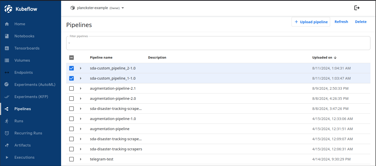
2. Click on a custom pipeline and select + Create run

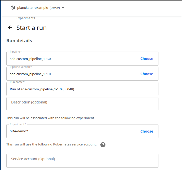
3. Configure the run:
- Leave pipeline name, version, and run name as default.
- Choose an experiment that is relevant to the run: this is purely organizational.
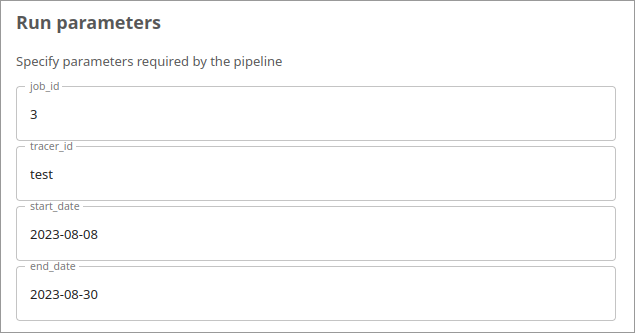
- Specify Input Parameters. Note: It's good practice to choose a new job_id every run.
- Click Start
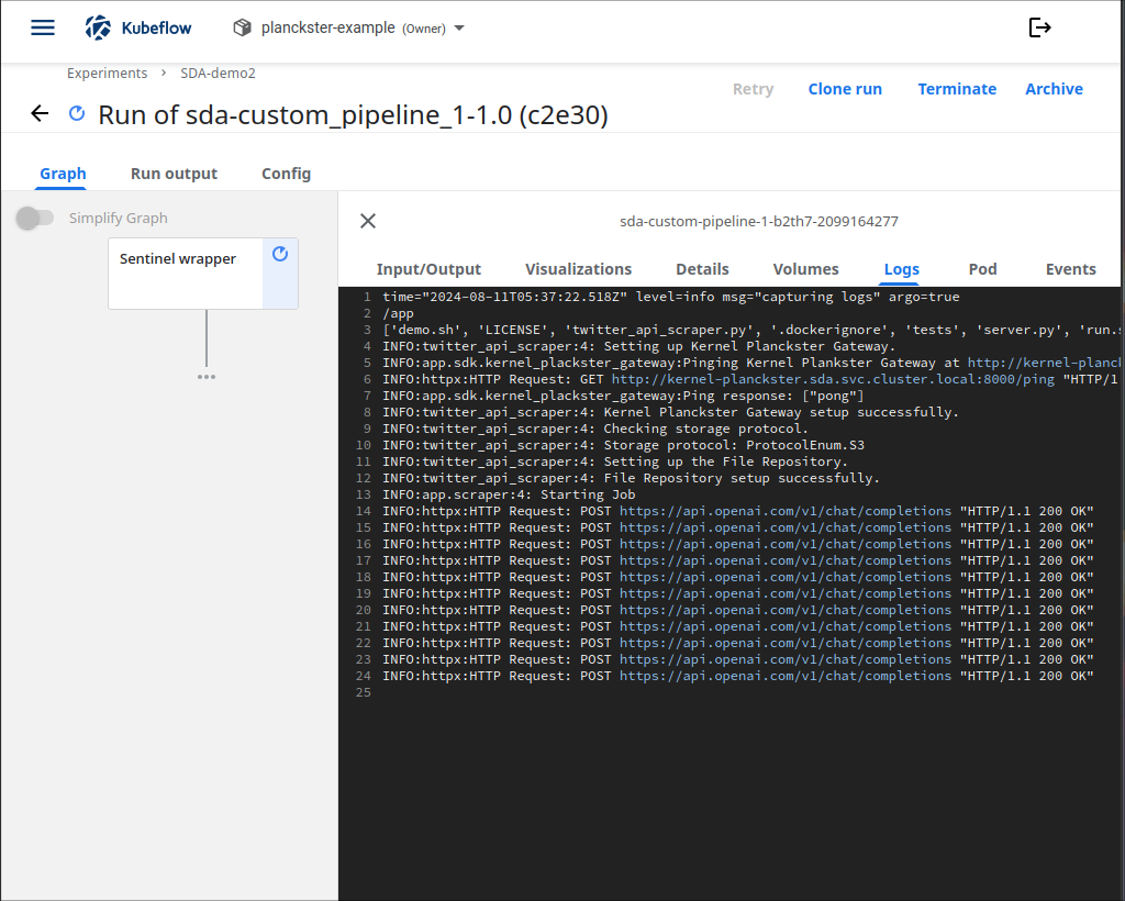
4. View logs:
5. Ensure successful job completion:
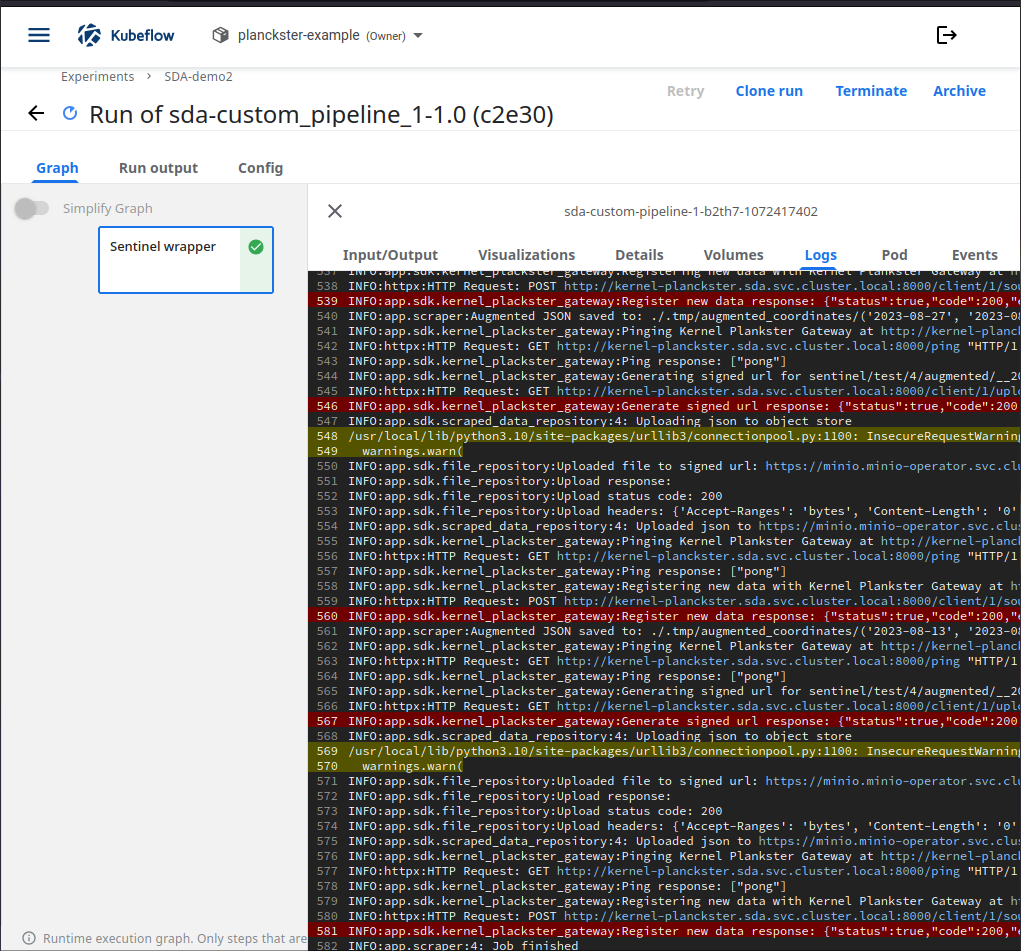
You should see the "Job finished" message at the end of the log page. Additionally, check the MinIO bucket to make sure all necessary data was uploaded.
Conclusion
You now understand how to create and upload custom pipelines by reusing previously defined components. This is a very powerful practice that allows for rapid testing of various configurations of workflows. When paired with custom augmentation, one can even analyze the same scraper data in different ways.